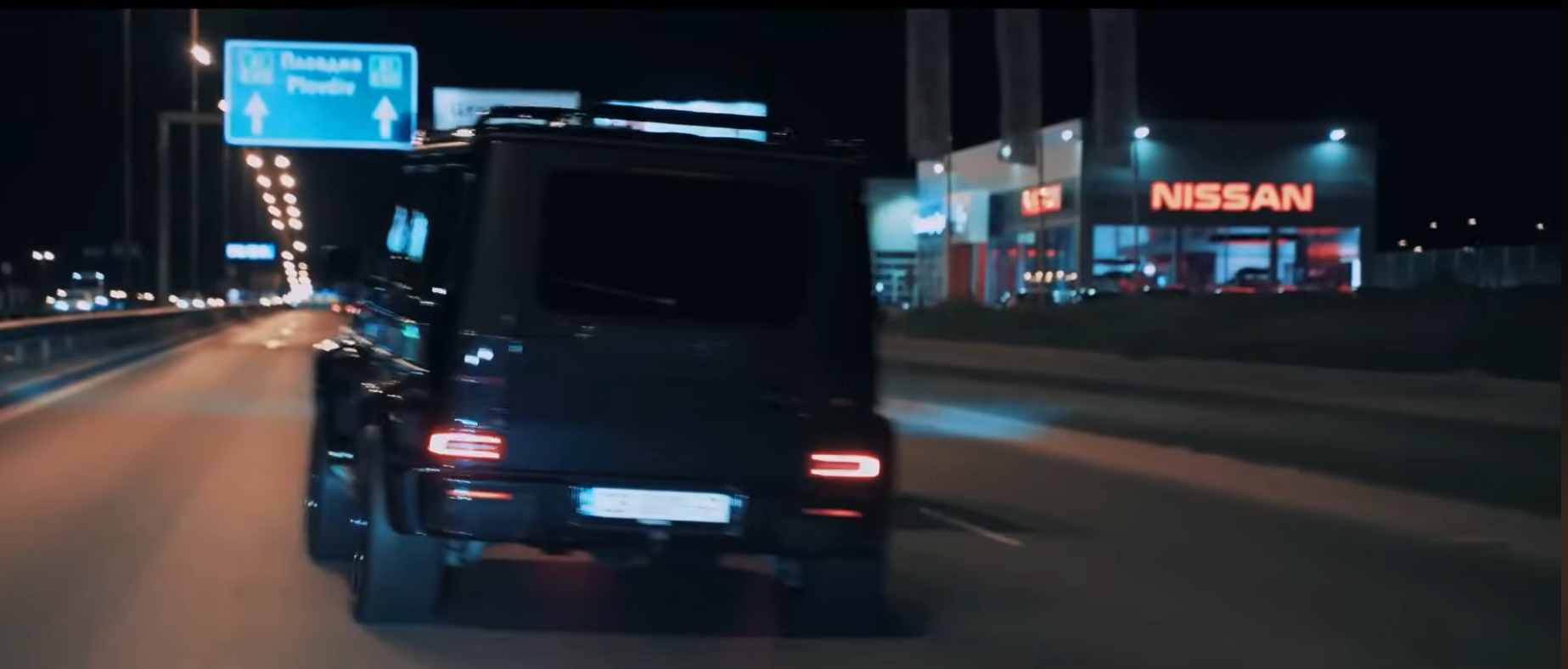
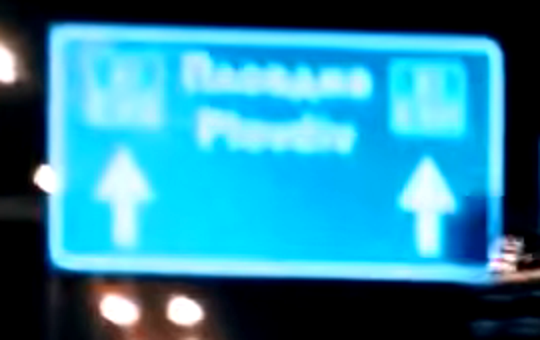
This page reconstructs the Python cells used to inspect and enhance the supplied night-driving frame: Pillow crops, OpenCV local-contrast experiments, route-sign pixel analysis, and a Richardson–Lucy deconvolution sweep. Failed experiments are retained because they are part of the actual worklog.
Spontaneous solution from GPT-5.6-Sol to a question about identifying the location of a highway.
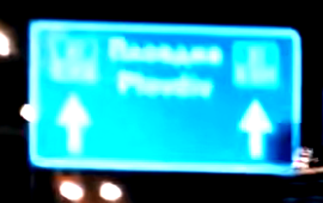
Try a different enhancement pipeline: cubic upscale, local contrast enhancement in LAB space, then an unsharp mask.
Python
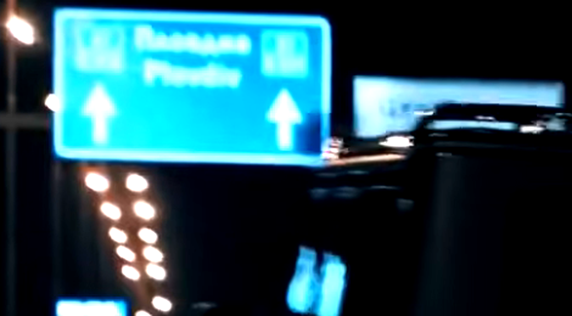
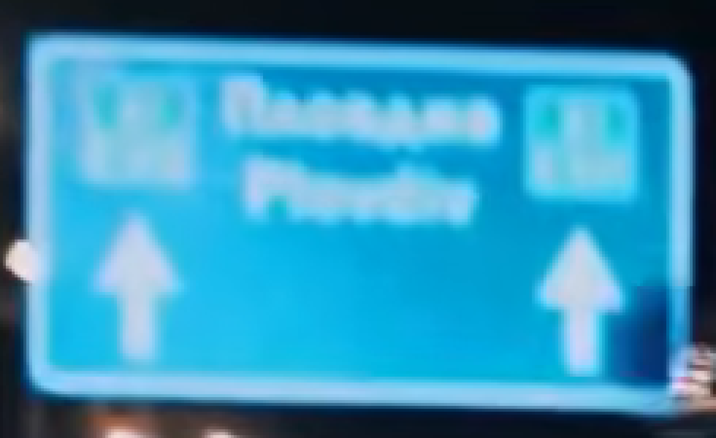
importcv2,numpyasnp,matplotlib.pyplotasplt,PIL.ImageasPImagearr=cv2.imread('/mnt/data/69b09c25-0e8d-48fb-8826-ae9405e6e49f.png')# sign region exactr=arr[45:220,240:680]# upscale nearest/cubic and unsharpup=cv2.resize(r,None,fx=5,fy=5,interpolation=cv2.INTER_CUBIC)# CLAHE on LABlab=cv2.cvtColor(up,cv2.COLOR_BGR2LAB)l,a,b=cv2.split(lab)cl=cv2.createCLAHE(clipLimit=2.0,tileGridSize=(8,8)).apply(l)enh=cv2.cvtColor(cv2.merge([cl,a,b]),cv2.COLOR_LAB2BGR)gauss=cv2.GaussianBlur(enh,(0,0),2)sharp=cv2.addWeighted(enh,1.8,gauss,-0.8,0)cv2.imwrite('/mnt/data/sign_cv.png',sharp)
Output
True
sign_cv.png
[5]
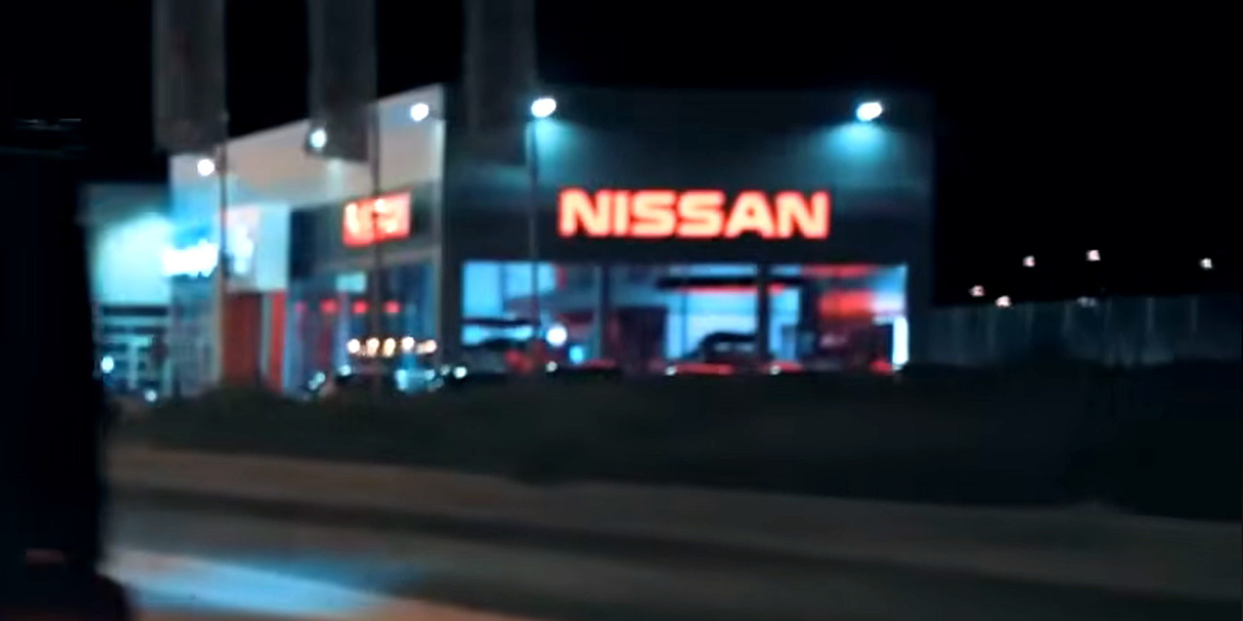
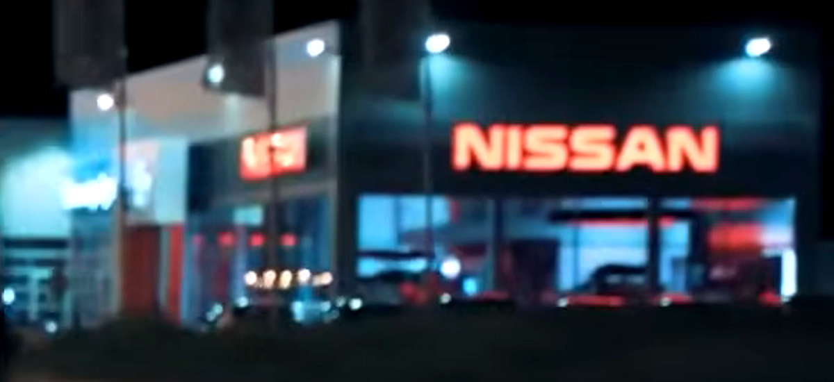
Enhance the dealership side of the frame
Crop the right-hand roadside businesses and boost contrast/sharpness to inspect logos, signage and facade geometry.
Create a deliberately blocky enlargement of the original sign pixels so blur structure can be judged without interpolation artifacts.
Python
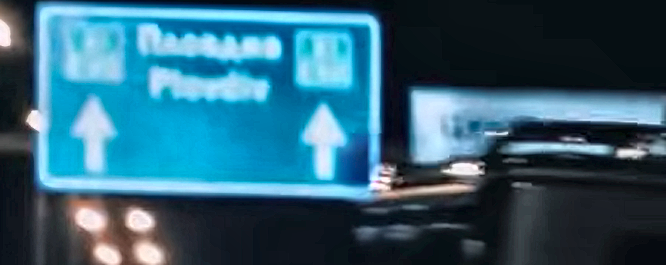
fromPILimportImage,ImageEnhance,ImageFilterimg=Image.open('/mnt/data/69b09c25-0e8d-48fb-8826-ae9405e6e49f.png')# crop sign more tightly original pixelscrop=img.crop((255,35,500,185))# nearest upscale 6xnear=crop.resize((crop.width*6,crop.height*6),Image.Resampling.NEAREST)near.save('/mnt/data/sign_nearest.png')print(crop.size)
Output
(245, 150)
sign_nearest.png
[10]
Check for scikit-image
Verify that scikit-image is installed before trying a deconvolution experiment.
skimage ModuleSpec(name='skimage', loader=<_frozen_importlib_external.SourceFileLoader object at 0x7f5fd7da26a0>, origin='/opt/pyvenv/lib/python3.13/site-packages/skimage/__init__.py', submodule_search_locations=['/opt/pyvenv/lib/python3.13/site-packages/skimage'])
[INTERLUDE]
Analyzed dealership signage and blurred text clues
Output
[11]
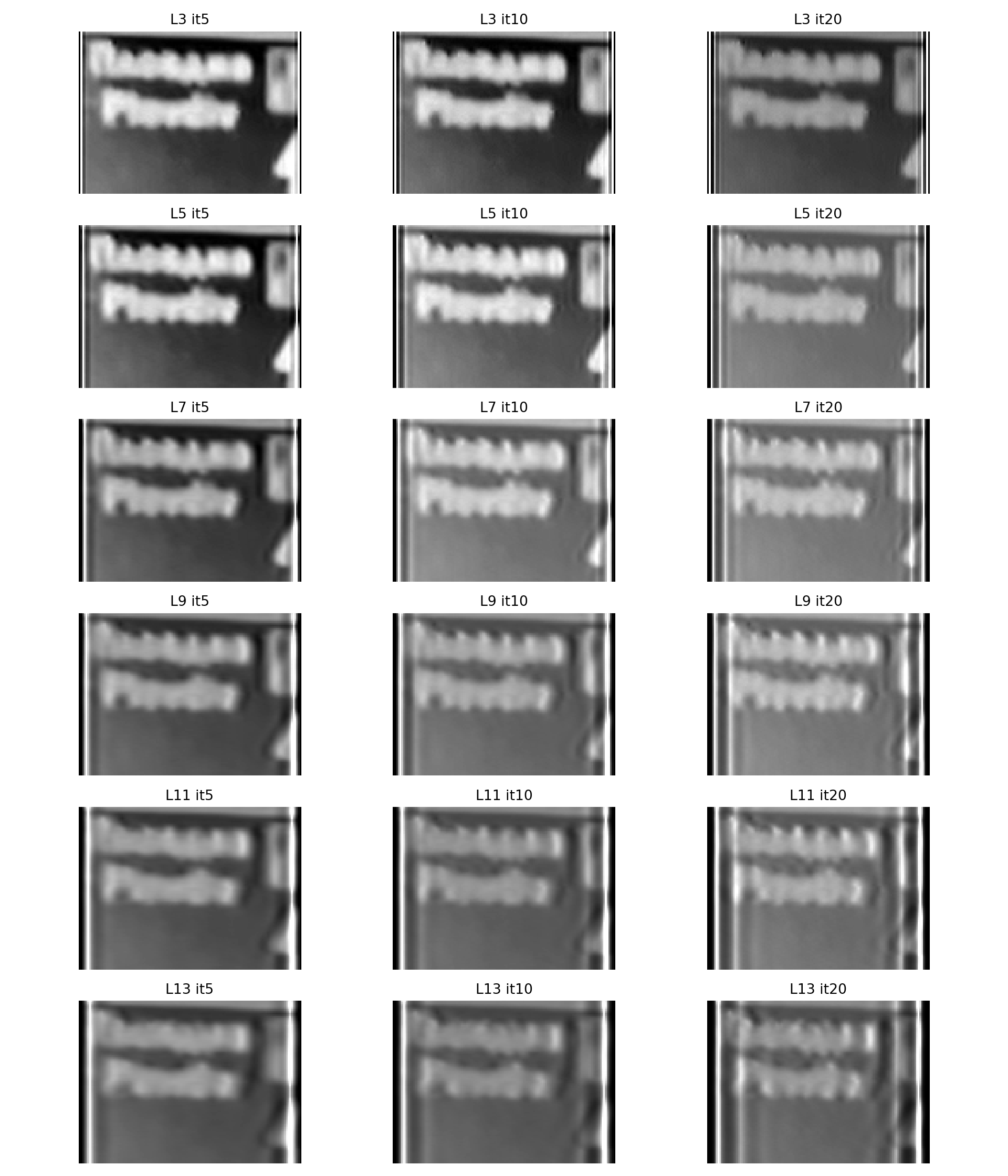
Richardson–Lucy deconvolution: first attempt
Sweep several horizontal blur-kernel lengths and iteration counts. This first version failed while rescaling the deconvolved intensity range.
Python
fromPILimportImageimportnumpyasnp,matplotlib.pyplotaspltfromskimage.restorationimportrichardson_lucyfromskimageimportexposureimg=Image.open('/mnt/data/69b09c25-0e8d-48fb-8826-ae9405e6e49f.png').convert('RGB')# text onlyc=np.array(img.crop((325,55,455,150)).convert('L'))/255.0results=[]forlengthin[3,5,7,9,11,13]:psf=np.zeros((1,length))psf[0,:]=1/lengthforitin[5,10,20]:de=richardson_lucy(c,psf,num_iter=it,clip=False)de=exposure.rescale_intensity(de,in_range=np.percentile(de,[2,98]),out_range=(0,1))results.append((length,it,de))fig,axs=plt.subplots(6,3,figsize=(12,14))forax,(l,it,de)inzip(axs.ravel(),results):ax.imshow(de,cmap='gray',vmin=0,vmax=1)ax.set_title(f"L{l} it{it}")ax.axis('off')plt.tight_layout()plt.savefig('/mnt/data/deconv_contact.png',dpi=200)
Output
ValueError: The truth value of an array with more than one element is ambiguous. Use a.any() or a.all()
Convert the source to NumPy and draw a grid over the sign region to estimate precise text-line coordinates.
Python
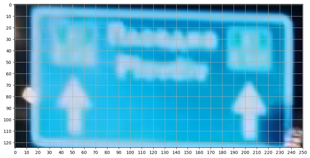
fromPILimportImageimportnumpyasnp,matplotlib.pyplotaspltimg=np.array(Image.open('/mnt/data/69b09c25-0e8d-48fb-8826-ae9405e6e49f.png').convert('RGB'))# approximate text line bounds from original# display sign coordinate with grid perhapsc=img[45:170,250:500]plt.figure(figsize=(15,6))plt.imshow(c)plt.xticks(np.arange(0,251,10))plt.yticks(np.arange(0,126,10))plt.grid()plt.show()
Output
Interactive Matplotlib output.
[15]
Column-brightness projections for the text lines
Use the red channel as a crude white-text detector on the blue sign and plot horizontal profiles to estimate where characters begin and end.
Python
importnumpyasnp,matplotlib.pyplotaspltgray=img.mean(axis=2)# lines orig coordstop=gray[65:87,338:430]# maybebot=gray[94:115,338:430]# whiteness relative to blue background: use R channel maybe text white = high R, background blue = low RR=img[:,:,0].astype(float)topR=R[65:90,335:435]botR=R[94:118,335:435]# projection positive after subtract median baseline per column? simple max or percentileforarr,namein[(topR,'top'),(botR,'bottom')]:prof=np.mean(arr,axis=0)# smooth?plt.figure(figsize=(12,2))plt.plot(prof)plt.title(name)plt.xticks(range(0,101,5))plt.grid()plt.show
Output
Interactive plots; the final line intentionally references plt.show without calling it, matching the original cell.
[16]
Measure color dominance in sign subregions
Compare RGB statistics in the two suspected route badges and central text area to see whether any route marker carries a distinct color.
Python
fromPILimportImageimportnumpyasnp,colorsys,pandasaspd,mathimg=np.array(Image.open('/mnt/data/69b09c25-0e8d-48fb-8826-ae9405e6e49f.png').convert('RGB'))# approximate sign bounding box x=262..494 y=47..169# examine badge regionsregions={'left_badge':img[55:115,270:330],'right_badge':img[62:120,425:485],'center_text':img[55:125,330:425],}forname,ainregions.items():# mean rgb and top chromatic pixelsflat=a.reshape(-1,3)print(name,flat.mean(0),flat.min(0),flat.max(0))# pixel proportions where red dominance or green dominancer,g,b=flat[:,0],flat[:,1],flat[:,2]print("red dom",np.mean((r>g*1.15)&(r>b*1.15)),"green dom",np.mean((g>r*1.15)&(g>b*1.05)),"blue dom",np.mean((b>r*1.1)&(b>g*1.05)))
Output
left_badge [ 83.97083333 191.10555556 230.00055556] [ 15 168 208] [180 210 249]
red dom 0.0 green dom 0.0 blue dom 1.0
right_badge [ 40.72988506 173.38477011 215.58132184] [  0 128 182] [191 214 249]
red dom 0.0 green dom 0.0 blue dom 1.0
center_text [ 63.30962406 181.15804511 224.63954887] [  0 129 185] [184 216 255]
red dom 0.0 green dom 0.0 blue dom 1.0
[17]
Top-hat morphology on the sign
Try isolating bright lettering from the blue background with a grayscale morphological top-hat transform, then save both grayscale and top-hat variants.
Python
importcv2,numpyasnp,matplotlib.pyplotasplt,os,PIL.ImageasIim=cv2.imread('/mnt/data/69b09c25-0e8d-48fb-8826-ae9405e6e49f.png')# sign regions=im[45:180,260:500]# channels perhaps use min? Text white on blue, grayscalegray=cv2.cvtColor(s,cv2.COLOR_BGR2GRAY)# subtract local background via morphological opening?# white features use top-hatkernel=cv2.getStructuringElement(cv2.MORPH_ELLIPSE,(15,15))tophat=cv2.morphologyEx(gray,cv2.MORPH_TOPHAT,kernel)# crop text lines# save variantsouts=[]fori,arrinenumerate([gray,tophat]):arr2=cv2.resize(arr,None,fx=6,fy=6,interpolation=cv2.INTER_CUBIC)ifi==1:arr2=cv2.normalize(arr2,None,0,255,cv2.NORM_MINMAX)cv2.imwrite(f'/mnt/data/sign_proc{i}.png',arr2)'/mnt/data/sign_proc1.png'
Output
'/mnt/data/sign_proc1.png'
sign_proc0.pngsign_proc1.png
[18]
Extract the two destination-text lines
Save tight top/bottom line crops using both nearest-neighbor and cubic interpolation for side-by-side visual comparison.
Python
importcv2,numpyasnpim=cv2.imread('/mnt/data/69b09c25-0e8d-48fb-8826-ae9405e6e49f.png')# let's save very tight text crop without badges# original sign around x260-500 y45-180. text top x333-423 y56-84, bottom x336-418 y86-114forname,y1,y2in[('top',55,86),('bottom',83,115)]:a=im[y1:y2,325:430]# upscale nearest and cubicformethod,labelin[(cv2.INTER_NEAREST,'n'),(cv2.INTER_CUBIC,'c')]:b=cv2.resize(a,None,fx=12,fy=12,interpolation=method)cv2.imwrite(f'/mnt/data/{name}_{label}.png',b)
Output
top_n.pngtop_c.pngbottom_n.pngbottom_c.png
[19]
Reload the original frame before another crop
Reinitialize the Pillow image object after NumPy/OpenCV experiments and confirm dimensions again.
Compute a simple mean-luminance profile across the sign to identify rows most affected by bright text, arrows and reflective elements.
Python
importnumpyasnp,matplotlib.pyplotasplt,pandasaspdarr=np.array(img)# crop original signsc=arr[45:185,260:500]# luminance?lum=sc.mean(2)# print rough rows/cols max averagesrows=lum.mean(1)[(i+45,rows[i])foriinnp.argsort(rows)[-20:]]
Calculate mean and median RGB values for small sign regions. This failed because the current image array had a channel shape incompatible with reshape(-1, 3).
Python
importnumpyasnpa=np.array(img)# show mean RGB for regionsregions={'leftshield':(270,55,323,114),'rightshield':(420,70,473,123),'bg':(330,60,390,100)}forname,(x1,y1,x2,y2)inregions.items():r=a[y1:y2,x1:x2]print(name,r.reshape(-1,3).mean(0),np.median(r.reshape(-1,3),axis=0))
Output
ValueError: cannot reshape array of size 12508 into shape (3)
[25]
RGB-region statistics: corrected conversion
Force the Pillow image to RGB before converting to NumPy, then recompute the region statistics successfully.